Presentation slides are available here

1 Introduction

This work is a review of (Li, Kang, and Hu 2013). It has been conducted as part of the validation process of the MVA lecture Introduction à l'image numérique [project description].

You may also want to check out a snapshot of my working notebook.

The next Section focuses on explaining the idea of the guided filter fusion as presented in the studied paper. Section 3 shows example of my implementation. Section 4 highlights some limitations of the proposed method. Section 5 give access to the code as well as an example of use. As an openning, Section 6 presents my willing to make this method more accessible and belief in node-based user interface through an integration to Blender compositing system.

2 Guided Fitler Fusion

The algorithm for image fusion using guided fitler, then called Guided Filter Fusion (GFF), is really well explained in the first sections of the studied paper. I will go here incrementally from the basic idea of merging to the final algorithm.

2.1 Basic merging

Let's say we want to merge two images I_A and I_B, whatever there is on them:

Image merging

Roughly, merging will consist in picking each pixel of the output image either from I_A or from I_B. More generally, the output will be a linear combination of both inputs: W_A × I_A + W_B × I_B where  ×  stands for the pixel-wise product.

Weighted image merging

As illustrated on the scheme, in most cases W_B = 1 − W_A, or almost. This may be important for some energy conservation.

GFF is no different from this simple merging and all the magic is in the definition of the weight matrix.

2.2 Saliency

In order to find the merging weights, also called masks when they are binary, GFF relies on the notion of saliency. Basically, the algorithm will want to pick the pixels from the input image which is locally the more detailed. The saliency map gives an actual definition to this qualitative idea. It is a measure of "detailness" based on the laplacian of the image. The higher the magnitude of the laplacian, the more detailed the picture. In order to spread this notion to the neighborhood of a pixel, the saliency map is blurred.

Then GFF compares the saliency of both input images and sets the output color as the color of the input image with the highest saliency. This can easily be extended to more than two images.

At this point, the weight W_A and W_B are just binary masks representing argmax(S_A, S_B) where S stands for the saliency map.

2.3 Guided Filter

The main issue of binary weights is that it introduces artifacts at the mask boundaries, jumping from one input image to the other one. The first idea to tackle this is to blur the masks, but one quickly notices that it breaks the sharpness of the mask in some areas in which it is needed.

In order to blur the mask while keeping details, GFF uses a Guided Filter (He, Sun, and Tang 2010). Other filters such as bilateral filter could be used. This makes the merging much less visible.

2.4 Multiscale

Finally, this kind of image processing is typically applied to different scales independently, decomposing the input images into a pyramid of levels of details, processing each of them independently, and then merging them back into the final output.

Multiscale weighted image merging

The paper pragmatically note that two level is far enough for most applications, making the algorithm much simpler than if there were an arbitrary number of them.

I won't go more into the detail of the algorithm, since the paper does it well. I will now move on examples.

3 Examples

I present here some examples of application of my implementation.

3.1 Fly

This first example uses the illustration image of the project proposal:

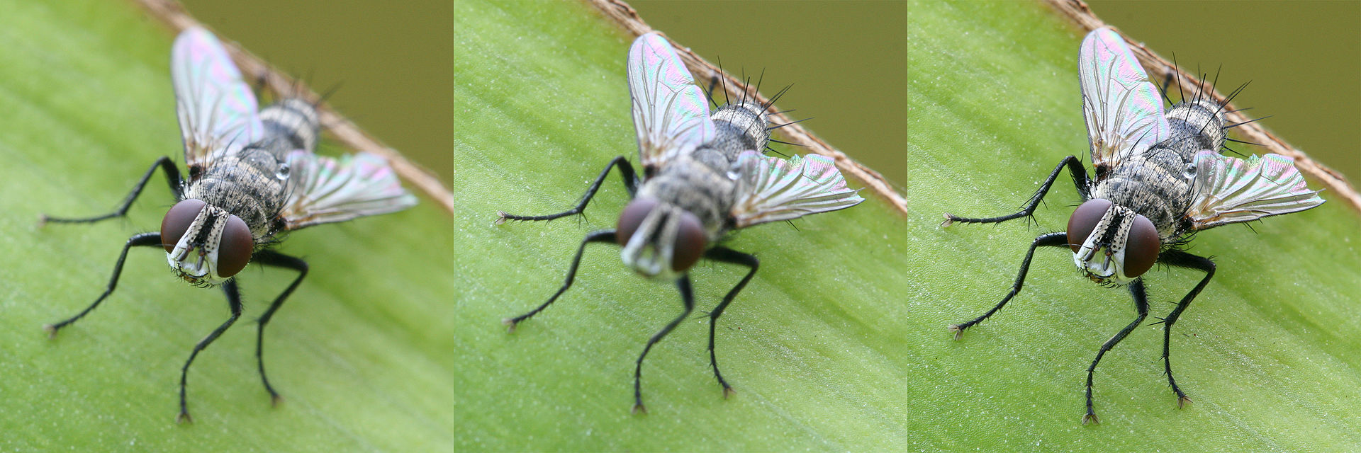
Fly shot under different Depth of Field settings

I used the first two images as input and tried to get something close to the third one. This is also the example mostly used in the notebook. Here are some examples of intermediary steps on a first grayscale test:

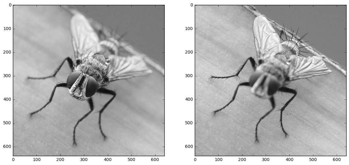
Input images

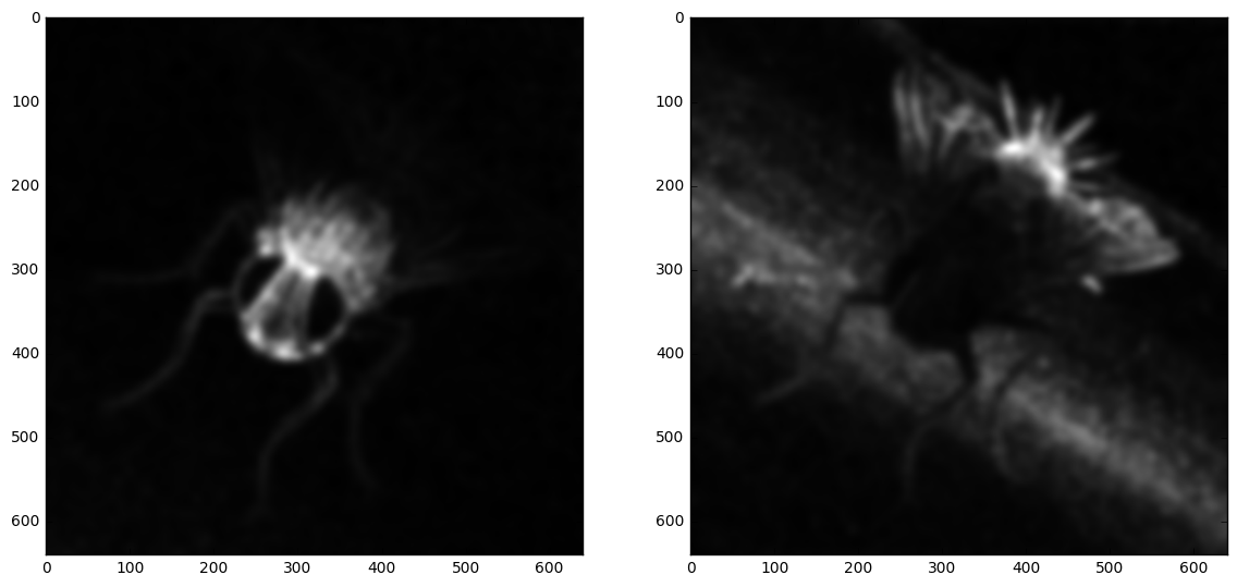
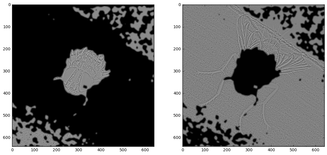
Saliency maps

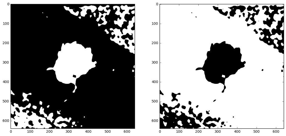
Masks, before guided filtering

Weights used for merging detail scales

Here is a final output for the colored fly:

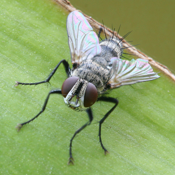
Merged fly

It is not as sharp as the reference image, but I highly doubt that the latter has been obtained by merging the first two. It is sharp in areas in which none of the first two is and is not perfectly registered. Yet, my result is really valuable compared to my input images.

3.2 Bookshelf

3.2.1 Input Images

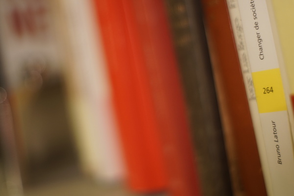
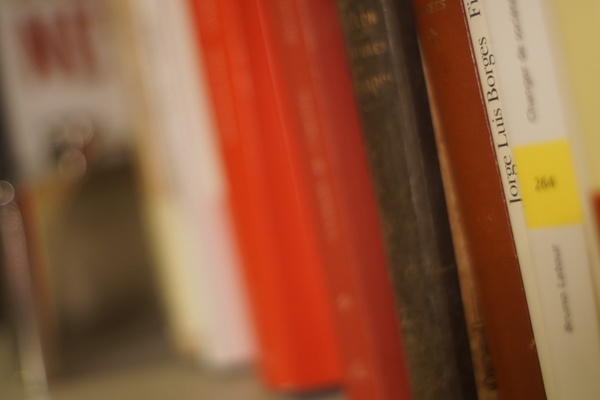
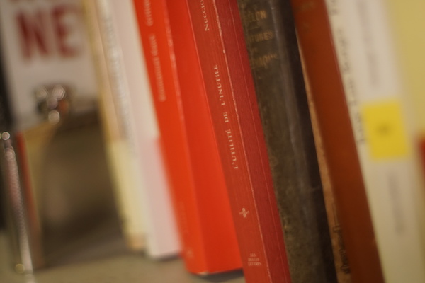
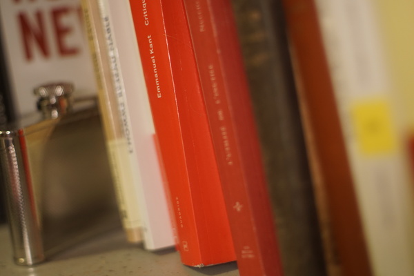
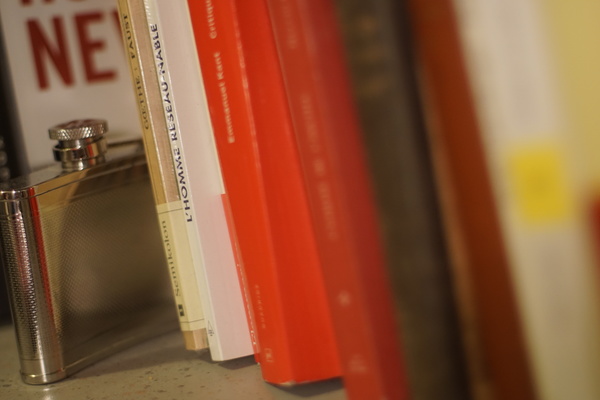
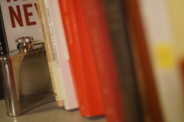
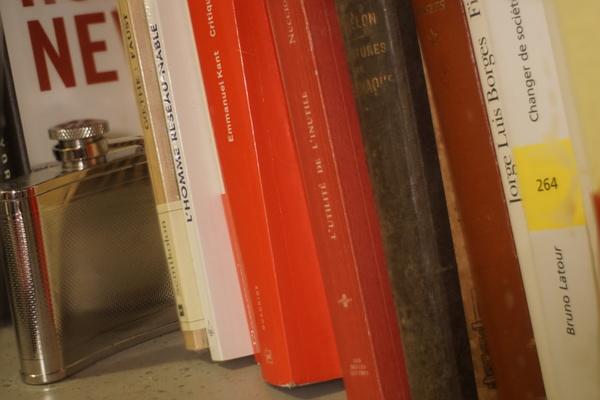
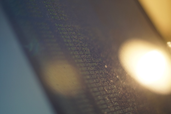
In order to test the merging capabilities of GFF for more than two images, I took several pictures of my bookshelf with a very local focus on the different books successively. This example is interesting because one can expect the mask boundaries to be aligned with books' sides. The ability to read the titles is a good criterion to determine whether the merging is satisfying.

These picture have been shot using a Sony a6000 mirrorless camera equipped with a 50mm lens at aperture f/1.4. A tripod has been used to ensure image alignment and the camera was triggered remotely to avoid shaking it while pressing the button. I had to touch it anyway between the shots to modify the focus because it is a fully mechanical lens. No digital registration has been performed: pictures are used as output by the camera.

bookshelf1

bookshelf2

bookshelf3

bookshelf4

bookshelf5

bookshelf6

bookshelf7

3.2.2 Results

3.2.2.1 Images 1 and 2 only

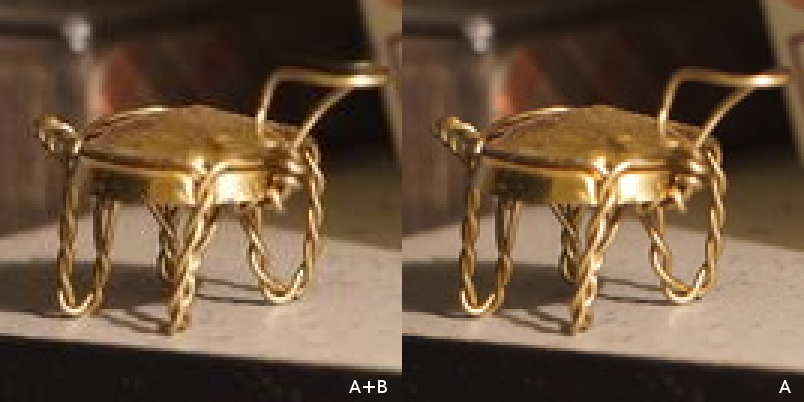
I first tried to merge two images only, as in previous tests.

Bookshelf 1+2 only

The resulting image is sharp where at least one of the input was sharp, so this part was correctly reconstructed and is it hence possible to read the first two titles, which was possible on neither on the input images.

Nevertheless, the left-hand side of the image, that was blurry in both inputs, has become noisier. If one looks carefully, one can notice that there are "sparkles" of both images. Since none of the input was sharp, it was hard to choose one of them. One can notice at least that there is some regularity in the choice. It would have been worst if the selected image would have been almost random.

3.2.2.2 All images

All bookshelf images merged

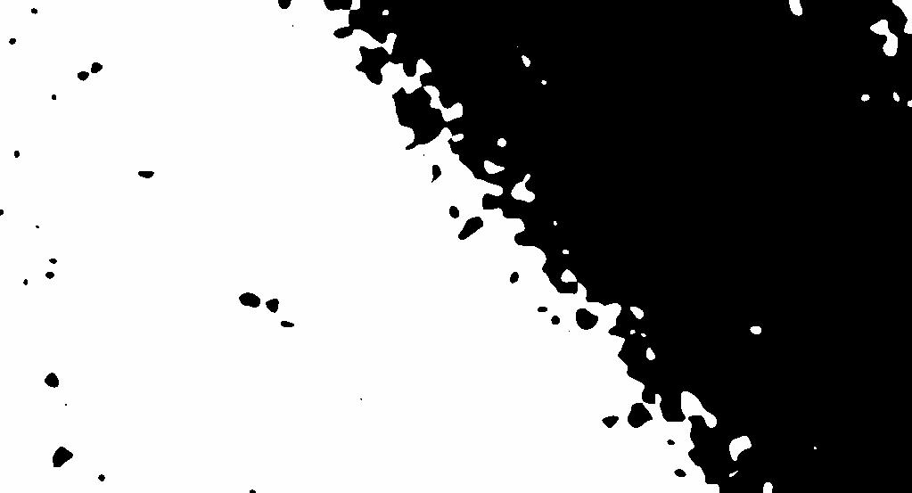
It is interesting to have a look at the mask map:

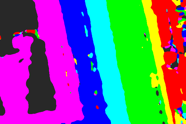
Bookshelf mask

Each color of this picture correspond to an input image and gives, for each pixel, which image has the more important saliency.

It is important to note that this map is not used as is for merging. Guided filter is then applied to it, with different parameters depending on the scale (base or details) as we have seen in Section 2

Most of the noisy parts of the mask map correspond to uniform areas of the final picture in which the choice of the input picture to consider is not that important, except for the traces around the number 264 of the right-most book. This is because the object does not feature a lot of detail in this area so it is hard without more advanced area recognition to know whether it is in focus or not.

To be honest, I was pretty amazed by this image. Despite its previously noted limitations, it really matches well what one could expect from the algorithm.

3.3 The crane and and the tutle

(This is not from La Fontaine)

The crane and and the tutle

This example is used in the next section to illustrate some limitations.

3.4 Screen reflexion

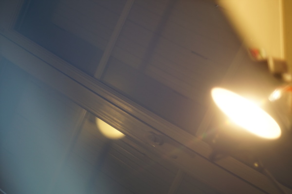
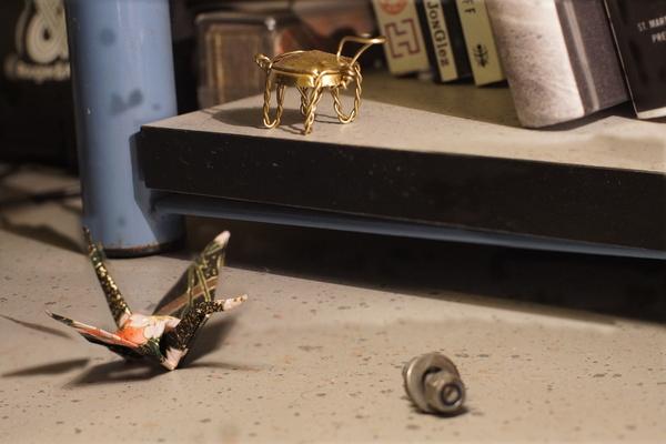
In order to trouble the algorithm, I build an example in which reflexion effects make the focus completely change the scene. The next two pictures are shot with the exact same pose but the first one focuses on the screen itself while the second one focuses on the wall reflected by the screen.

Naturally, the result is terrible. Taking reflexions into account is clearly out of the scope of this method.

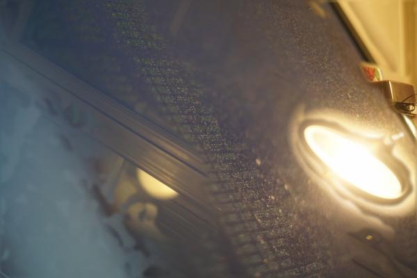
Fusion with reflexion

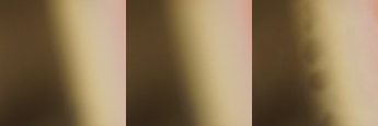
Here are the saliency maps of the four merged images:

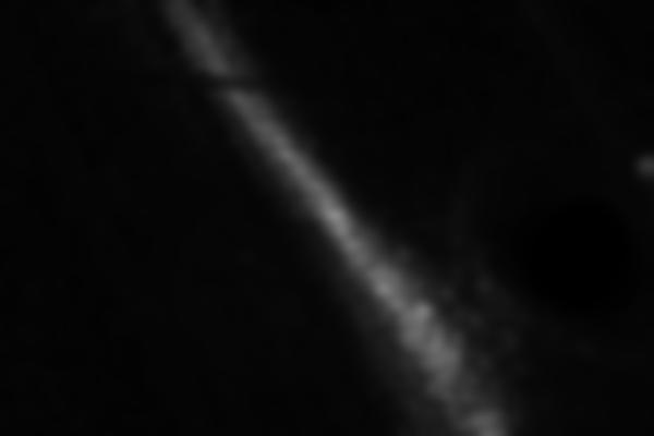
Saliency map 1

Saliency map 2

Saliency map 3

Saliency map 4

The merging on the screen only worked well:

Fusion of two pictures of a screen

Associated mask

4 Limitations

We have already seen some limitations through the examples.

4.1 Indecision in blurry areas

When merging only the first two bookshelf images, the out-of-focus area was not correctly merged because none of the input images was very "convincing" for the maximum of saliency.

Artifact introduced by the algorithm in an area that has high regularity (sample of bookshelf 1+2)

Interestingly, the bokeh effect reduces this indecision by introducing sharper borders, because bokeh is a non gaussian blurring effect. Hence, the fusion suffers from less artifacts where the bokeh is marked.

4.2 Reflexion

Though the example that I gave was a bit extreme, such reflexion phenomenon may introduce artifacts. This is a problem of many image processing algorithms by the way, because reflexion breaks a lot of hypothesis of invariance.

4.3 Misalignment

Even when assuming that the camera did not move at all between the shots, changing the focus usually introduces a distortion in the light path, which zooms in/out a bit and may change the radial deformation. This is particularly visible in the crane and and the tutle, especially on the shadows because since shadows are smooth, the mask boundary may cut them and take half of it in an image and the other half in another one.

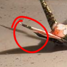
Broken shadow due to imperfect image registration

4.4 Noise highlight

The method relies on basic saliency map and so has a certain tendency to highlight noisy areas, like compression noise.

Jpeg compression artifacts highlighted by the fusion

4.5 Robustness

The pictures used as input must not only be correctly registered but also need to be taken under the same settings, especially lightning.

The crane and the turtle, where light source has been moved between the two images.

The crazy shadow is particularly representative of the problem that a change of lightning can create, but even slighter changes may have important consequences on colors, as it is here on the ground whose white tone changes. It is hence highly recommended preprocess the images with at least some histogram equalization (Pizer et al. 1987).

5 Implementation

I first wrote my own implementation following only the studied paper, in order to check that it completely describes the method. All the previous examples have been made using this implementation.

5.1 Code

As already mentioned, you can follow my steps of development and get detailed examples in my working notebook. If you just need a standalone version, it holds in two files:

• imagerie.py: utility fonctions related to image processing but not guided filtering fusion itself
• fusion.py: the guided filtering and fusion implementation

It is very easy to use. For instance:

from fusion import imread, cGFF, imwrite

A = imread("A.jpg")
B = imread("B.jpg")
C = imread("C.jpg")

fused = cGFF([A, B, C])

imwrite("fused.jpg", fused)

You can feed an arbitrary number of input images to merge to the algorithm.

I apologize for the lack of documentation of the proposed code. As for now, I consider that the notebook is a first approximation of documentation and so I let myself publish this code despite my love for clean code. Let me know (at ) if you intend to use it and would make it cleaner. It is released under the MIT license, by the way.

5.2 Requirements

I tested my code using Python 3¹. The only requirements are:

• numpy/scipy that any scientific user of Python is likely to have
• matplotlib, as likely to already be on your system and required only for the visualization, so not mandatory

5.3 Performances

I did not recorded precisely the computing time, plus it depended on the machine I was using (which varied), but it was all "human time", meaning that it was reasonable to run it and wait for it to finish without feeling the need to have a coffee in the meantime. Roughly it was taking 20s for the 7 bookshelf images, which are 600×400 px. I ran out of my 4GB of memory when running it on images higher than 2000×2000 px.

I did not focus on performances in this implementation. I was more concern with it in the C++ implementation for Blender that comes in Section 6.

5.4 Other implementations

The authors of the paper released their own implementation, in MATLAB. A link is available at http://xudongkang.weebly.com/ [direct link].

A quick search pointed me to an explicit implementation of the same paper, also using Python but with the opencv binding: fuse-img. The use of OpenCV binding in this context is a bit overkill: it does not make it easier to implement as a pure Python solution but if one would want to make the filter available in OpenCV -- which would be great -- Python is not teh best way to go. Implementing it in C++ would be a more robust choice. The guided filter has already been cleanly implemented here so it would be quite straightforward to implement full GFF.

Although I considered doing this OpenCV implementation, I finally focused on another implementation, as presented in the next section.

6 Integration to Blender compositing nodes

6.1 Node-based editing

As many algorithms of image processing, or even more generally of signal processing, the GFF method is intuitively represented as a flow-based processing graph. This representation is so common that it is at the heart of the User Interface of many advanced tools such as 3D softwares (Maya, Houdini, Blender^{[open source]}), video compositors (Nuke, Natron^{[open source]}), texture generators (MaPZone, Substance Designer), and so on.

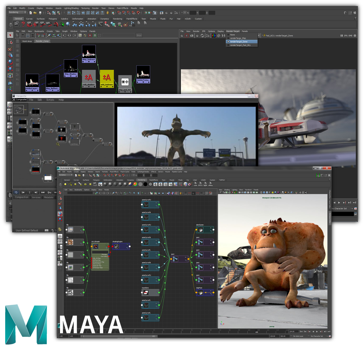
Node-based workflows in Maya

Houdini is fully procedural and represents anything under the hood as a node.

The Foundry's Nuke also represent all operations as nodes, which is more flexible than After Effect's layers.

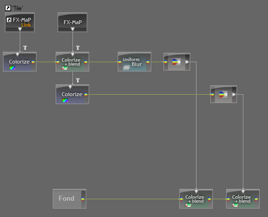
Node layout describing a texture in MaPZone, which has unfortunately been discontinued by Allegorithmic to focus on Substance

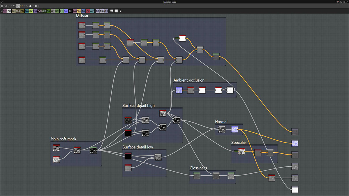
Substance Designer fundamentally relies on nodes in order to describe fully parametric fractal-based textures.

Beyond the flexibility it introduces for the graphical user interface in signal processing applications, computation graphs are at the heart of bleeding edge research frameworks such as Theano and TensorFlow because they are essential for operations such as automatic differentiation.

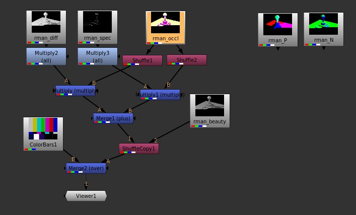
The studied paper itself presents its method through its computation graph. It is hence natural to want to implement it in a similar way.

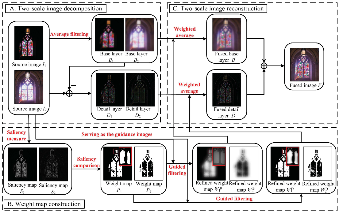
Node-based representation of the algorithm as presented in the studied paper

I have been myself really convinced by this approach for a long time and though many times about a generic way of implementing many of my personal projects as node graphs. So I wanted to benefit on the occasion created by this project to focus a bit on one of these node systems.

Instead of reinventing the wheel, I knew that I had first to have a deeper look at the existing solutions, and two open source were interesting candidates. Even if I would eventually consider building a generic node-based editor from scratch, getting some experience with existing tool is a good way to think about their design and the main challenges.

6.2 Open source candidates

Even though closed source softwares such as Nuke provide very flexible API for building new nodes, I feel more comfortable working with open source softwares. The two major candidates that I hence considered where Natron and Blender.

6.2.1 Natron

Natron is a quite young video compositing software largely based on The Foundry's Nuke, even up to its look n feel. It has been first known in 2013 by winning Inria's Boost Your Code challenge and it has been actively supported by the Inria since then. First attracted by its fully node-based workflow, I was also happy to learn that it is a product of French scientific research.

Its similarity to Nuke was made possible by the Open Effects initiative to standardize interfaces between image processing filters in the Visual Effects (VFX) industry. This was led, among others, by The Foundry which put a lot of its own design in it. Although it was mainly intended to make proprietary filters banks and compositing softwares communicate better, it also fostered open source initiatives.

Hence I considered implementing the GFF algorithm as an OpenFX Plug-in. This would have made it available not only in Natron but also in Nuke and numerous other so-called OpenFX hosts.

6.2.2 Blender

Blender is the open source reference of 3D software suite. It is incredibly full of features ranging from 3D modeling to 3D rendering and compositing, including animation, texturing, physic simulation, etc. It has been more and more used in professional VFX and has demonstrated its numerous qualities through a sequence of open movie projects.

Blender uses node-based editing for 3 different purposes:

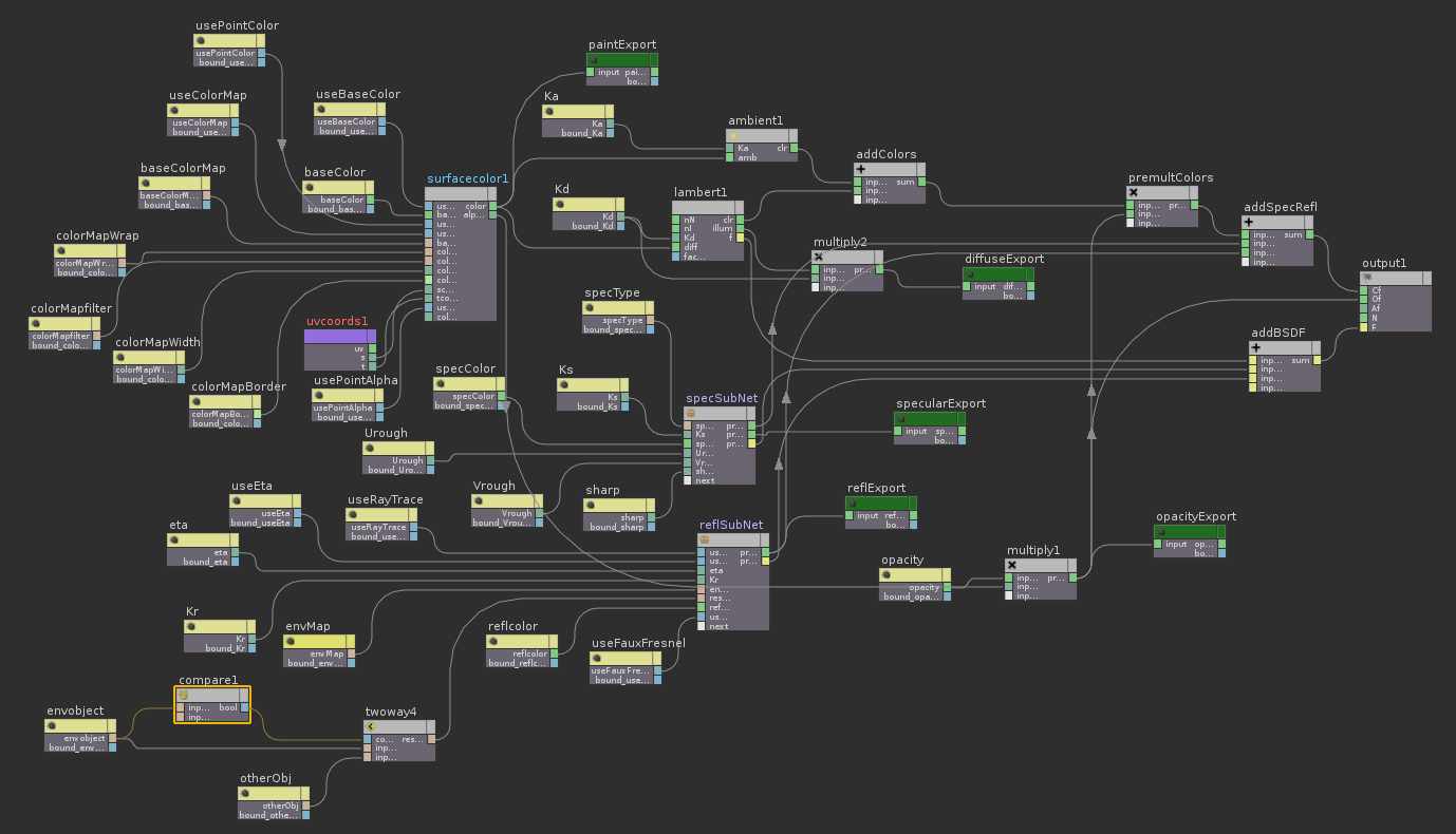
• Shader definition: The recent Cycle render engine uses node graphs to describe the interaction of casted light rays with the matter.

• Texture generation: Blender features a procedural texture generation interface based on nodes. Unfortunately, it is not as advanced as Substance's one and maybe underused.

• Compositing: Maybe the first use of nodes in Blender, chronologically speaking. Similarly to Nuke or Natron, compositing nodes implement 2D processing algorithms applied posterior to rendering.

What was missing to Blender to be able to reproduce the paper's processing graph in Blender compositor was a the Guided Filter². All the other blocs were already available. Furthermore, I have much more experience with Blender than with Nuke/Natron and I had been wanting to know more about Blender coding for a long time. So I choose to focus on Blender first.

6.3 Writing a new compositing node for Blender

When it comes about extending Blender's capabilities, its Python API is usually the way to go. It is rooted deep into Blender's architecture and enable hence clean and powerful interaction with the existing software bricks. Unfortunately, the node creation is an exception, so I had to fork the code and edit C/C++ files.

I mostly followed Nazg-gul instructions which was almost exhaustive about what to do on the "piping" side³. And I managed to get my node implemented.

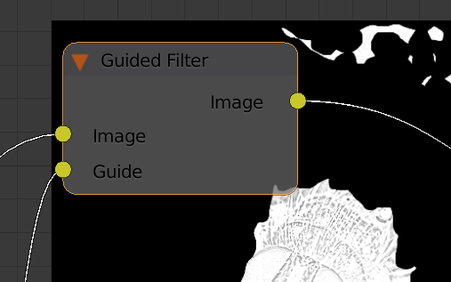
Guided Filter node

You may note that the node is missing faders to set epsilon and the kernel size. This is just a UI issue, these parameters are accessible through the command line.

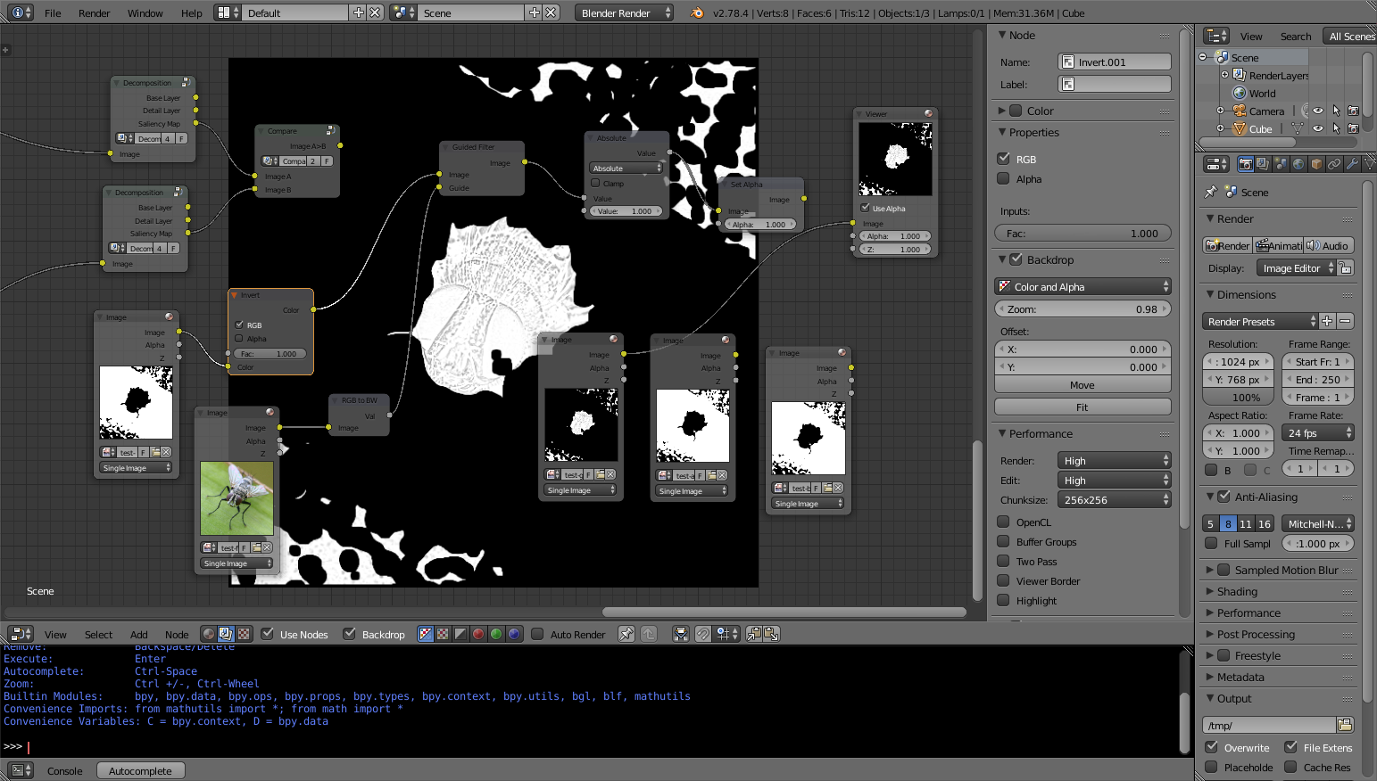
Experimentation in Blender compositor around the Guided Fitler node

The output of the node suffers from some artifacts that I suspect to be caused by NaNs and is more generally not completely what I would expect, but the basic idea is here and it can already be used.

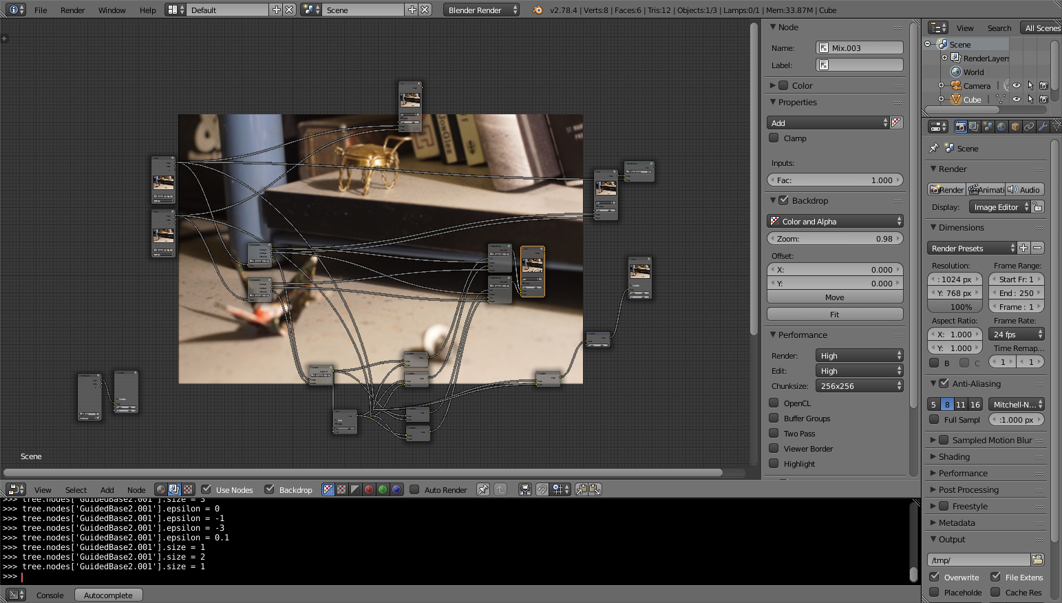
Guided Filter Fusion in Blender Compositor

This part is still a work in progress but I am already happy with the work accomplished and my first tangible change to Blender code. This implementation is also much more efficient than the Python implementation and makes the fusion almost real time.

7 Conclusion

Merging images using Guided Filter is a pragmatic algorithm for image fusion that is at the same time visually plausible and easy to implement in different contexts.

Making Guided Filter available in an interactive procedural image processing application such as Blender compositor is a way to tackle the imperfection of the fusion algorithm by enabling a user to edit its different steps on the fly. The computational simplicity of GFF makes this process very interactive.

This project was for me an exploration of the image processing algorithm itself and a state of the related tools and projects.

8 References

(See also all the hyper-links inside the report.)